How can the optical path of a distributed fiber optic temperature sensing (DTS) system be integrated into a single enclosure?

2026-07-18 11:00:20

Keywords： DTS Optical Path Integration

Overview

Manufacturers, system integrators, and university research teams looking to develop distributed temperature sensing (DTS) systems often face the following challenges: purchasing pulse lasers, WDM multiplexers, dual-channel APD detectors, and high-speed data acquisition cards separately; assembling four-channel optical switches individually; performing fiber splicing and optical path coupling and debugging; resulting in messy hardware cabling, poor optical path consistency, and bulky equipment. R&D teams spend the majority of their time on optical path matching and hardware integration, diverting critical personnel who should be focusing on temperature demodulation algorithms and industry-specific host software.

YBphotonics has launched the DTS Integrated Module (Model: GY-DTS-M), which fully integrates the laser, WDM, APD, and 250M high-speed data acquisition card. This solution handles the underlying DTS optical path and signal acquisition in a single step, allowing the R&D team to focus exclusively on demodulation algorithms and industry-specific software development—reducing costs, accelerating development, and simplifying mass production all at once.

Integrated Design: All DTS Optical Path and Acquisition Hardware Packed into a Single Enclosure

The module features highly integrated internal components, including a 1550 nm pulsed laser, a Raman WDM wavelength division multiplexer, a dual-channel APD photodetector, and a 250 MSps high-speed acquisition card. Upon receipt, users can immediately obtain complete raw optical signals for both Stokes and anti-Stokes components.

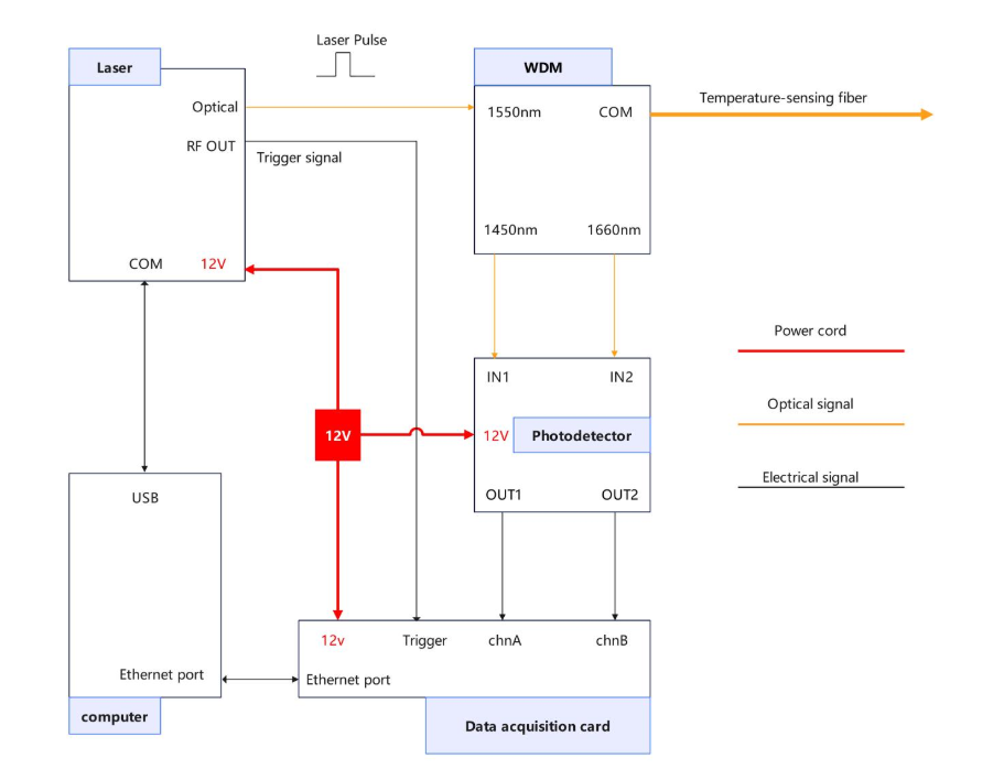
Built-in Reference Fiber and Temperature Output

The device includes 100 meters of built-in reference fiber and collects real-time temperature data via a temperature sensor, facilitating demodulation for users.

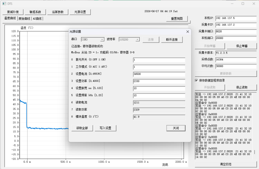
UDP Gigabit Ethernet output, minimal development, with a focus on algorithms and software

The module uses a standard Gigabit Ethernet port and the UDP protocol to transmit raw acquisition data. No additional hardware drivers are required, and it is compatible with any programming language. You can use Python, C, C++, Java, C#, LabVIEW, or other languages you are familiar with to acquire and demodulate data:

The module can directly output two channels of raw Raman scattering waveforms (Stokes / anti-Stokes) via the UDP protocol;
R&D teams can optimize their proprietary demodulation algorithms based on the raw signals, develop industry-specific host applications, and integrate with cloud platforms to achieve high-precision DTS using their own demodulation methods;
For customers without demodulation capabilities, we also provide YBphotonics’ temperature calculation demo software. By configuring the cloud platform’s endpoint in the software, the demodulated temperature curves can be posted to your cloud platform via the HTTP protocol. The cloud platform then simply needs to receive, store, and display the data via its UI.

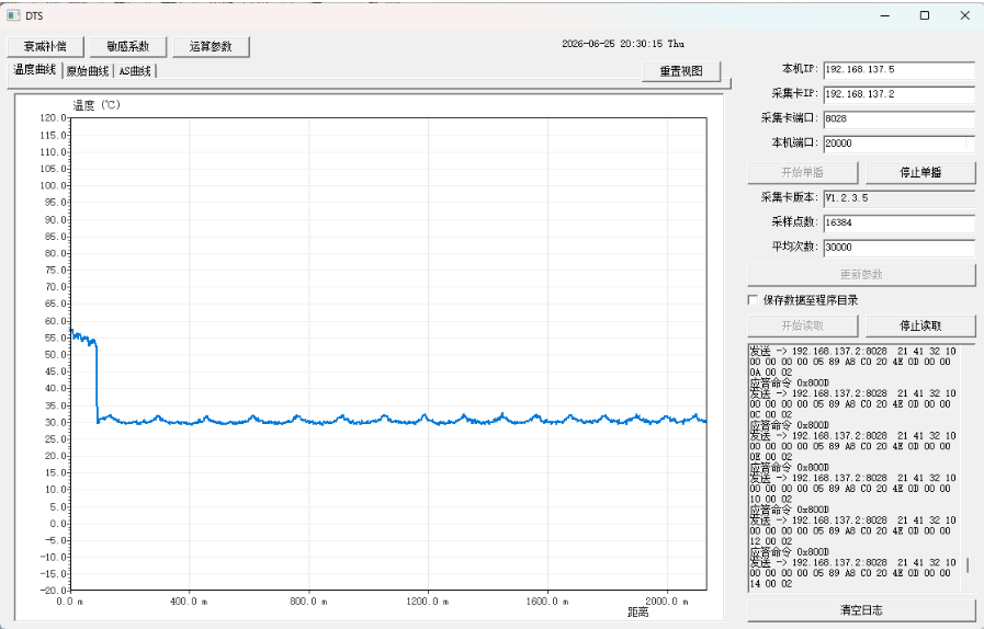
Robust, industrial-grade specifications that meet the requirements of long-range temperature measurement projects spanning 10 km

Key Performance Indicators	Parameter Details
Monitoring Distance	10 km
Center Wavelength	1550.12 nm, maximum peak output power of 30 W
Spectral Width (20 dB)	0.3 nm
Repetition Rate	Adjustable from 5 to 20 kHz, pulse width from 5 to 120 ns
Sampling Specifications	250 MSps sampling rate, 0.4 m sampling accuracy
Operating Environment	-15°C to 55°C wide-temperature operation, 9–13 V DC power supply, total power consumption 13 W
Sensor Pigtail	62.5/125 multimode fiber, FC/APC connectors, fiber output length ≥ 1 m

Screenshot of the DTS Module Test Report

1. Example Diagram of Laser Pulse Width Modulation

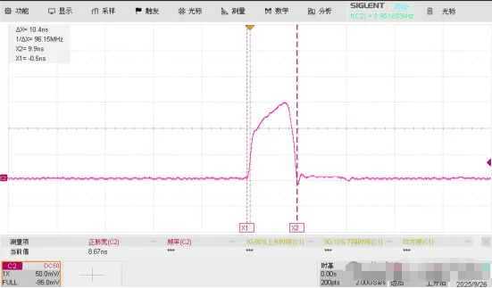
1.1. Set the frequency to 10 kHz and the pulse width to 5 ns; after connecting the laser module to a photodetector, the oscilloscope display appears as shown in the figure below:

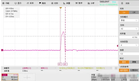
1.2. With the frequency set to 10 kHz and the pulse width to 10 ns, the following waveform is displayed on the oscilloscope when the laser module is connected to the photodetector, as shown in the figure below:

2. Raw Stokes and Anti-Stokes Curves from the DTS Module

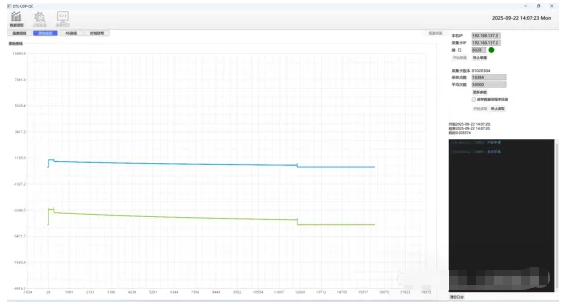
2.1. Set the frequency to 10 kHz, the pulse width to 5 ns, and the fiber length to 5 km. The raw curves acquired by the software are shown in the figure below:

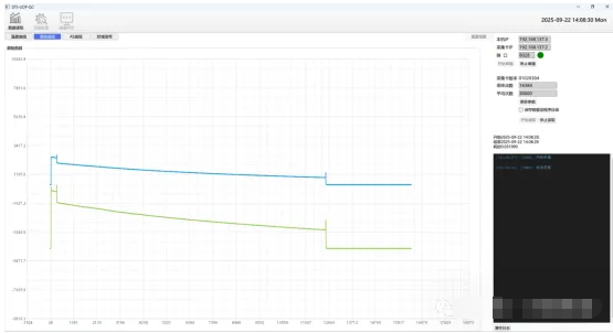
2.2. Set the frequency to 10 kHz, the pulse width to 10 ns, and the fiber length to 5 km. The raw waveform captured by the software is shown in the figure below:

Experimental Data from the Solution Software

We developed a temperature solution program (which performs only simple averaging and noise reduction, without using complex wavelet-based noise reduction) and obtained the following experimental data; if your demodulation algorithm is more advanced, you can certainly achieve even better results.

Parameter Item	Setting Value	Notes
Fiber Length	5000m	62.5/125 Temperature-Sensitive Optical Cable
Average Count	30000次
Repetition Frequency	10kHz
Pulse Width	10ns
Test Results
Parameters	Parameter Values	Notes
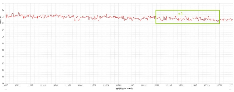
End-point noise	±1℃
Temperature accuracy	±1℃
Spatial resolution	1.2m

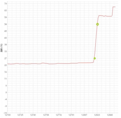
End-point noise: The lowest point in the green box is 22°C, the highest point is 24°C, and the noise margin is ±1°C.

Spatial resolution: Refers to the effective spatial distance along the fiber length during the sensing process. At the location of a disturbance, the fiber length corresponding to the range of 10% to 90% of the step change in the disturbance signal measured by the distributed fiber optic sensor is defined as the spatial resolution fiber length. As shown in the figure below: the 90% coordinate of the temperature-sensing coil is (12823, 54), and the 10% coordinate is (12820, 27). Therefore, the spatial resolution is calculated as (12823 – 12820) × 0.4 = 1.2 m.

Temperature accuracy, as shown in the figure below:

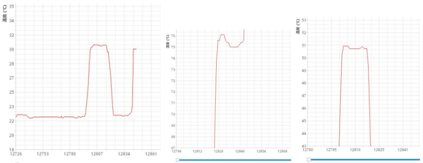
Temperature of the Constant-Temperature Water Bath (°C)	YBPhtonics Simulation Software Readings (°C)
30	30（±1）
50	50（±1）
75	75（±1）